Tweet-to-tweet learning

Natural language processing is arguably one of the most interesting application of machine learning. Recurrent neural networks are by far the most successful models in this context, with LSTM and GRU networks being the top choice.

One can find several excellent tutorials and blog posts on how to train a recurrent neural network on a text corpus. I would definitely recommend reading “The Unreasonable Effectiveness of Recurrent Neural Networks” from A. Kaparthy for a review of cool applications of RNNs.

Deep learning frameworks such as Keras and PyTorch also provide extensive documentation on how to build such a model.

In this post, I describe an experiment at building a system that learns the distribution of tweets scraped from the web and serves the results through a web interface. I will therefore go through all the OSMN (read “awesome”) steps that a data science typically project encompasses.

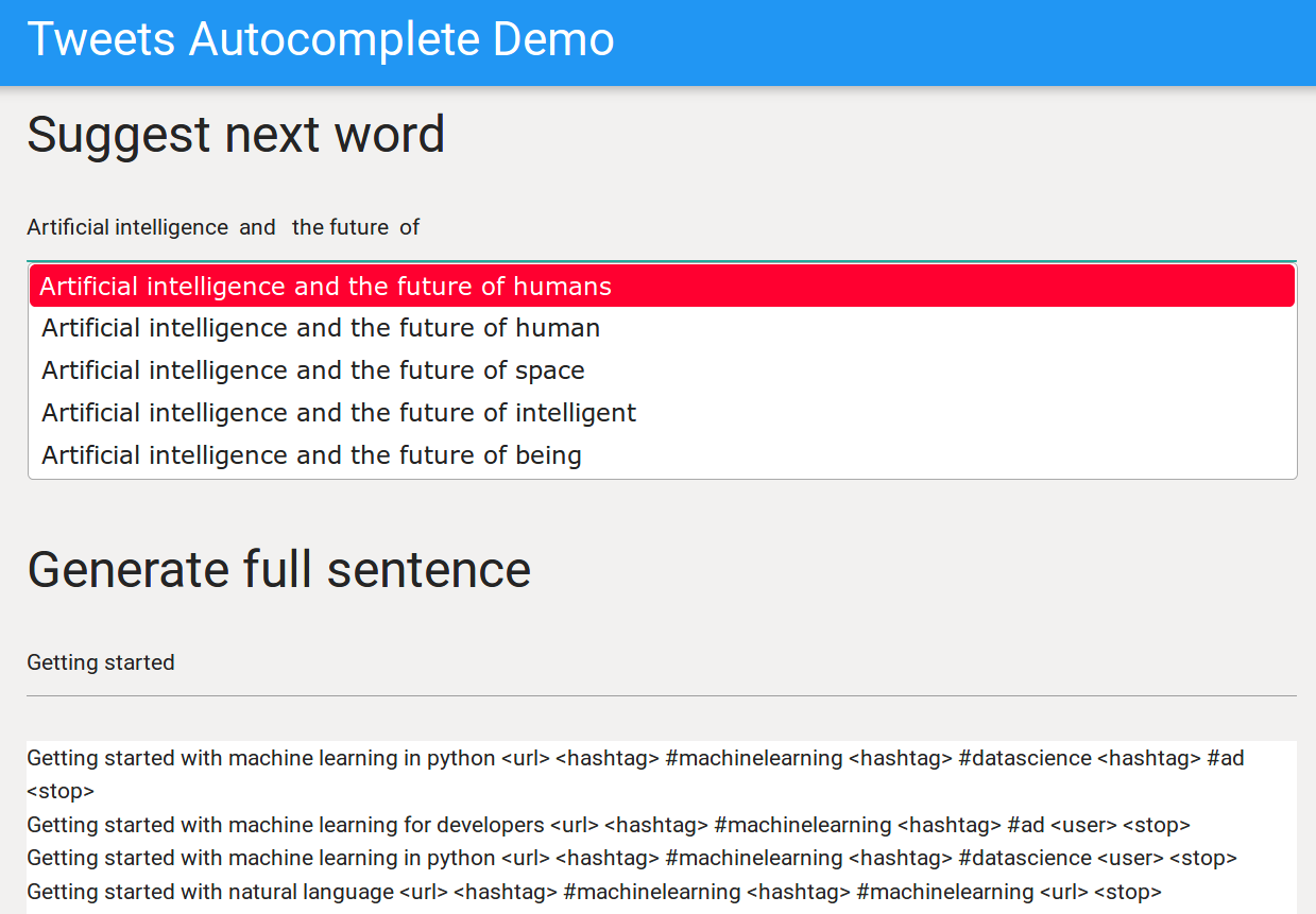
If you are curious to poke around the code, you can find it here. By clicking on the image below you can also check what the model predicts after being trained on a stream of tweets containing the hash tags #machinelearning and #neurips2018.

Here is the list of ingredients that we will need to get to the final result:

1. We will first have to scrape the data from the web and build the text corpus on which we will train the language model.

2. Afterwards, we will have to work out a suitable representation for the language data. Sententences are typically represented as sequences of words, which in turn are represented as fixed-size vector, through the so-called words embedding models.

3. At this point we will be able to train a language model. Recurrent neural networks based are state-of-the art for this purpose, and this is what we will use.

4. Once the model is trained we will use it to build an tweet auto-completion web application.

Collecting and cleaning the data

Building the tweet dataset from scratch requires a bit more effort than downlowading a pre-assembled dataset from the web. On the other hand, being able to mine the web is a skill that a data scientist should acquire if he/she wants to “create value from data”.

As I said, for this project I assembled a set of tweets related to machine learning, choosing the hashtags #neurips2018, and #machinelearning.

Once the raw data are collected, one needs preprocess and clean it up in order to allow the machine learning algorithms to digest them. This is a relative tedious process that is however crucial. As any good data scientist knows, 90% of the performance of a machine learning model depends on the quality of the input data.

Streaming tweets

So how can we download the tweets? The short answer is “using the tweetpy library”. To access the tweets one needs to apply for a developer account on twiiter and register an app. Once the account is created and the app registered you will need to generate and take not of you API keys and of the access tokens: they will be needed for authentication.

The free version of the twetter APIs come with a limit on the rate of requests to the server at around 300 requests per 15 minutes… not very large is you would like to download 100k tweets. To go faster one can use the so-called streaming API through which one subscribes to a set hash tag and/or users.

The tweet_streamer.py script opens the stream and dumps the received tweets to json files. You will need to store the authentication data in a file called config.yml that needs to contain the following fields:

consumer_key: <your_consumer_key>
consumer_secret: <your_consumer_key_secret>
access_token: <your_app_access_token>
access_token_secret: <your_app_access_token_secret>

Once authenticated, we can subscribe to the tweets stream and register a listener that will dump the tweets to files.

l = StdOutListener()
auth = OAuthHandler(consumer_key, consumer_secret)
auth.set_access_token(access_token, access_token_secret)

stream = Stream(auth, l,tweet_mode="extended")
stream.filter(track=['NeurIPS2018','MachineLearning'])

Preprocess and clean

Great: the tweets are being streamed to our hard drive! The next step is to load this data, clean it up and preprocess it, in such a way that it can be feed to the language model that we will construct. Text from tweets is quite peculiar, both because of the length limitation and because it contains a bunch of non-textual characters, in particular emoticons.

While emoticons contain relevant information to the meaning of a tweet, modelling it requires to developed a dedicated embedding. While this is conceptually no different from the treatment of hash tags that I describe below, fro the first iteration of this project I simply ignored this information.

The data pre-processing and cleaning is stirred by the preprocess.ipynb notebook. The twitter API returns the tweets data in JSON format. The tweet text is contained in the text field in the 140 character version, that is possibly truncated. In some cases the full text is also provided as a subfield of the extended_tweet field.

The first step is to load all the interesting data fields from the downloaded tweets and store them in a suitable data structure, such as a pandas DataFrame.

def load_all_tweets(path,
	keys=["id","text","lang","retweeted","retweet_count","truncated",
	"user/name","retweeted_status/extended_tweet/full_text",
	"extended_tweet/full_text"],lang="en"):
    tweets = glob.glob(path+"/tweet_*.txt.gz")

    filter_lang = (lang is not None and lang != "")
    if filter_lang and not "lang" in keys:
        keys.append("lang")

    df = pd.DataFrame( [ info for info in map(lambda x: extract_info(x,keys), sorted(tweets)) if info is not None ] )
    if lang is not None and lang != "":
        df = df[df["lang"] == lang]

    return df

After that, we apply a text preprocessing step that comprises the following steps:

1. Remove non-word characters from the tweets.
2. Expand contracted forms.
3. Perform pattern matching to identify know entities, such as numbers, hash tags, numbers and urls.

Here is an example of how the preprocessing and cleaning step transforms a tweet:

• original
  Relevance of #AI #SearchEngine in Business Processes\n\nhttps://t.co/0JoJdI6pgr\n\n#MariaJohnsen #BusinessIntelligence #SEO #smartweb #blockchain #Crypto & ofcourse 👉 #MachineLearning https://t.co/jtmwyiBy8Z

• preprocessed
  Relevance of <hashtag> #ai <hashtag> #searchengine in Business Processes <url> <hashtag> #mariajohnsen <hashtag> #businessintelligence <hashtag> #seo <hashtag> #smartweb <hashtag> #blockchain <hashtag> #crypto amp ofcourse <hashtag> #machinelearning <url> <stop>

We still have some work to do in order to obtain a clean and usable dataset. First of all, not all the tweets that we downloaded were unique, for two reasons: one is that the streaming API can actually send us the same tweet several times if we stop and restart the client, the other is that the same tweet can be retweeted many times. Before proceeding further, we want therefore to remove these duplicates.

Once all duplicates are removed, the tweets corpus is ready. We can now look into its word content. If we histogram the number of occurrences for the words in the dictionary, we find out that 10% of the text corpus is made by very rare words, that in turn account for 90% of the dictionary. If the training dataset is relatively small, the model may have a hard time at modelling such words. It turns out that one can actually be better off by ignoring the low-frequency words, as this allows to largely reduce the model complexity.

After preprocessing, I ended up with a corpus of roughly 30k tweets, and a dictionary of 2500 words, which cover 90% of the corpus.

Words representation

Representing words as geometric vectors is, in my opinion, one of the nicest and most effective tricks in NLP. The idea dates to the paper by Rumelhart et al. and it was first scaled up to dictionaries in the milions words size by Mikolov et al. in their word2vec paper.

Embedding a word dictionary consists in defining a mapping from the dictionary space to a vector space. The power of this approach is that semantic and grammatical relations between words can be represented efficiently by geometric relations. This is achieved by training a linear model to reproduce the words association patterns in the input text corpus. If you are interested to read more about words embedding, I would advice (besides googling the topic) to read this interesting blog post.

From the practical point of view, training an efficient words embeddings is a very computing intensive task and requires processing very large text corpora. Fortunately, pre-trained embeddings can be downloaded from the web. The most popular choices are the word2vec, GloVe and fastText embeddings.

For this experiment, I chose the GloVe embedding, because the authors provide an embedding trained on tweet data, that comes very handy if you want to work with tweets. The pretrained embedding does not know about hashtags, therefore I trained a dedicated one for hashtags using the tweet corpus that I collected for the this experiment. Since I was going to use GloVe for the text embedding, I also generated a GloVe embedding for hashtags. To do this, I first of all extracted the hashtags from the tweets. The input corpus was thus built by the sequence of hashtags in each tweet.

The GloVe approach to words embedding consists in building a model of the words co-occurence over the text corpus. Two words are said to co-occur if they appear within a fixed window from each other in any of the corpus sentences. The co-occurence matrix $X_{ij}$ counts the number of times two words co-occur in the whole corpus. Compared to the CBOW and skip-gram word2vec model this has the advantage of including information the global corpus statistics (hence the name).

In fact, the model focuses on the ratios of the co-occurence matrix, that is proportional to the likelihood ratio for pairs of words to be associated to each other. The model can be thought as a weighted least square regression on $\log(X_{ij})$. Its loss function is

$J = \sum_{i,j=1}^V f(X_{ij}) \left ( w_i^T \tilde w_j - \log(X_{ij}) \right )^2 $

Where the indexes $i$ and $j$ run over all the words in the dictionary, the vectors $w, \tilde w \in \mathbb{R}^d$, and the $i$-th word vector is $v_i = w_i + \tilde w_i$, and the function $f$ has the purpose of regularising the $\log(X)$ divergence and of weighting the importance of the different co-occurence matrix elements. Details on the derivation of this loss function can be found in the GloVe paper.

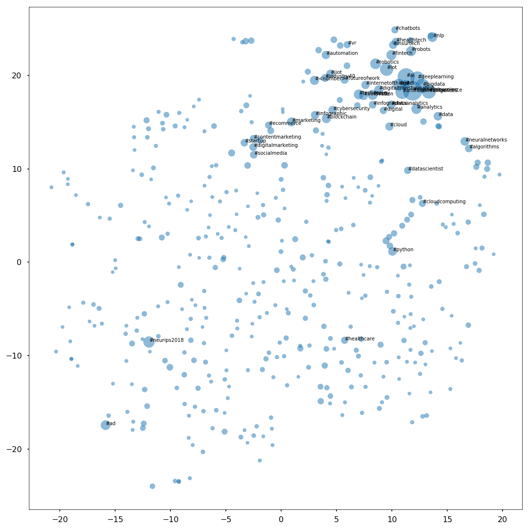
Enough for the introduction. In practical terms, I trained a 5-dimensional embedding for the hashtags and used a window of $\pm 5$ words for the co-occurence calculation. In this step I reused the code that is distributed by the GloVe authors. The shell script that I used to run this step is hash_embed.sh.

To visualize the result of the embedding, I used the t-SNE technique to reduce the dimensionality to 2. The t-SNE representation of the hashtags embedding is reported below. The size of the circles represents the hashtags frequency, and text labels are given for the most common ones.

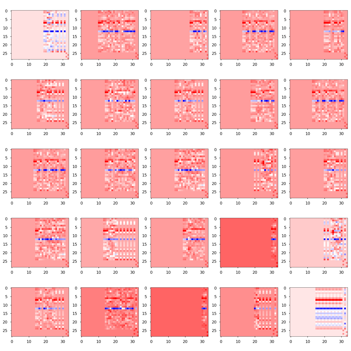
We have now all the ingredients needed to efficiently represent the tweets. The overall dimensionality of the embedding is 32: 25 dimensions are for the GloVe words embedding, 5 are for the hashtags, and 2 are used to mark unknown words and the end of sequence.

The image below shows the representation of a few sentences. The x axis corresponds to the sequence index (sequences are left-padded to 35 entries), the upper rows in y correspond to the GloVe embedding space, while the lower ones correspond to the hashtags embeddings.

Learning the sequence distribution

Now that we have constructed a suitable representation for our sequences, let’s tackle the problem of learning their distribution. What we will formally do is to estimate the density of tweets $t \sim p(t)$ over the tweets space $\mathcal{T}$.

A tweet is a sequence of words $t = \left ( y_1, … y_n \right ), y_i \in \mathcal{D}$, where $\mathcal{D}$ is the dictionary. We will factorise $p(t)$ as

$p(t) = p(y_1, …, y_n) = p(y_1) \cdot p(y_2\vert y_1) \cdot p(y_3\vert y_2, y_1) … \cdot p(y_n \vert y_{n-1}, …, y_1 ) $

and train a recurrent neural network to estimate $p(y_i \vert y_{i-1}, …, y_1 )$. The distribution $p(y)$ is discrete, and it can be parametrised a multinomial distribution. In particular, we want to find $\hat p_i(y_j \vert \vec \theta )$ such that

$p( y_j = i \vert y_{i-1}, …, y_1) = \hat p_i(y_j \vert y_{i-1}, …, y_1, \vec \theta )$

where $\vec \theta $ are the model parameters and $i$ enumerates all the words in $\mathcal{D}$.

Given our factorisation, the kind of recurrent network that we will train is a many-to-1.

The code to train the network can be found in notebooks/train_rnn.ipnb. I coded the network in keras and trained the model on the google colaboratory service.

As discussed above, the embedding space is factorised into three subspaces: the words embedding, the hashtags embedding, and the stop/unkown word annotations.

inp = Input(X_padded.shape[1:])

W = words_embed_layer(inp)
H = hash_embed_layer(inp)
S = stop_layer(inp)

L = Concatenate()([W,H,S])

For the network architecture, I chose to use two-layers of GRU units, that are faster to train than LSTMs, followed by three fully connected layers and a soft-max output layer.

To regularise the network, I inject gaussian noise at the input layer and at the level of the first and third fully-connected layer.

# recurrent layers
L = GaussianNoise(0.1)(L)
L = GRU(500,return_sequences=True)(L)
L = GRU(500,return_sequences=True)(L)

# fully-connected layers
L = TimeDistributed(Dense(250))(L)
L = GaussianNoise(0.05)(L)
L = Activation('tanh')(L)

L = TimeDistributed(Dense(250))(L)
L = Activation('tanh')(L)

L = TimeDistributed(Dense(250))(L)
L = GaussianNoise(0.05)(L)
L = Activation('tanh')(L)

# output layer
L = TimeDistributed(Dense(nwords))(L)
L = Activation('softmax')(L)

out = L
embed_model = Model(inputs=inp,outputs=concat)

The model obtains a top-1 (top-3) categorical accuracy of roughly 40(50)%, even though I did not spend much time tuning it.

Samples of predicted words can be generated during training. Below I put two examples obtained after 30 and 90 epochs, respectively.

epoch	30
input	can	blockchain	technology	save	the	environment	<url>	<hashtag>	#learning	<url>	<stop>
top-1 prediction		<hashtag>	<unk>	to	<unk>	<unk>	<url>	<hashtag>	#machinelearning	<hashtag>	<stop>
top-2 prediction		you	<hashtag>	<unk>	machine	future	in	<url>	#ai	<stop>	<url>

epoch

90

input

calling

all

marketers

ai

for

marketing

and

product

innovation

is

now

available

this

non

tech

guide

to

<hashtag>

#ai

<url>

top-1 prediction

all

<hashtag>

are

how

getting

goals

data

of

check

a

available

in

article

<unk>

<unk>

<url>

<url>

#machinelearning

<url>

<stop>

top-2 prediction

<hashtag>

<user>

can

in

free

strategies

analytics

<url>

today

out

on

for

post

<number>

<number>

read

learn

#datascience

<stop>

w

Generating sequences with beam search

Now that we trained our model, how can we use to predict tweets? A straighforward application is obviously to use it to suggest the next word while typing a tweet. This can be achieved simply by evaluating the model on the first part of the text to obtain the most probable next word.

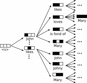
If we instead want to complete the full tweet starting from an intiial stub, we would need to compute joint probabilities over many word positions to select the most probably sequence. This would imply running a search over a tree with a branching factor equal to the number of words in the dictionary, which is clearly unfeasible.

A common solution is to construct an approximate using beam search. Beam search is a breadth-first search algorithm that, at each step, expands only the top-N combinations according to some heuristic function. In our case, the heuristic function will be the joint probability of the candidate sequences.

Let’s fix the beam width (i.e. the number of combinations that we will consider to 2).

• In the first step, the beam search will choose the two most probable words, according to the model, say $\hat y_{11}$ and $\hat y_{12}$, each with an associated probability $\hat p_{11}(s)$ and $\hat p_{12}(s)$ (where $s$ is the stub).

• In the second step, we will evaluate $\hat p_j(s,\hat y_{11})$ and $\hat p_j(s,\hat y_{12})$. For each of these these two candidate sequence we will choose the two most probable words $\hat y_{111}, \hat y_{112}, \hat y_{121}$ and $\hat y_{122}$. We will now choose the two most probable sequences according to the joint esitated probabilites $\hat p_{1i} \cdot \hat p_{1ij}$

• We repeat the previous step until all sequences end with a stop word (or the maximum number of iterations is reached).

Te implementation of the the algorithm is here.

    # ------------------------------------------------------------------------------------------
    def predict_next(self,seqs,log_probs0,nsuggestions):
        """ Expand the next search level and return candidate sequences
        
        Arguments:
        seqs        -- set of sequences currently in the beam
        log_probs0  -- log-probabilities associated to the current sequences
        nsuggetions -- number of suggested sequences to return (= beam width)
        Returns 
        candidates -- list of most probabile nsuggetions sequences
        log_probs1 -- associated log-probabilities 
        """

        # check which sequences have already a stop word
        candidates = []
        log_probs1 = []
        seqs_to_extend = []
        log_probs0_to_extend = []
        for seq,log_prob0 in zip(seqs,log_probs0):
            if seq[-1] == self.stop_word:
                candidates.append(seq)
                log_probs1.append(log_prob0)
            else:
                seqs_to_extend.append(seq)
                log_probs0_to_extend.append(log_prob0)
                
        ## print( self.tk.sequences_to_texts(seqs_to_extend) )

        # run the model prediction for sequences that have not yet ended
        if len(seqs_to_extend) > 0:
            X = pad_sequences(seqs_to_extend,self.padto)
            probs = self.model.predict(X)[:,-1,:]
            if self.unk_word is not None:
                probs[:,self.unk_word] = 0.

            # extract the top nsuggestions for each sequence that needs to be expanded
            preds = np.flip(probs.argsort(-1)[:,-nsuggestions:],-1)
            # expand the current sequences with the new suggestions and compute the
            # corresponding log-probabilities
            for seq, log_prob0, pred, prob in zip(seqs_to_extend,log_probs0_to_extend,preds,probs):
                seq = seq
                for ipred in pred:
                    ilog_prob = np.log(prob[ipred])
                    candidates.append( seq+[ipred] )
                    log_probs1.append( log_prob0+ilog_prob )

        # extract and return the nsuggestions with largest log-probabilities
        log_probs1 = np.array(log_probs1)
        keep = np.flip( log_probs1.argsort(-1)[-nsuggestions:], -1 )
		
	return [ candidates[icand] for icand in keep], log_probs1[keep] 

Wrapping it all up in web application using Flask

Ok. We are now ready to wrap everything up and serve our predictions, using for example a web application. The Flask microframework can be efficiently used for this.

Flask allows to quickly develop web application serving dynamic content with python as the underlying engine. For this experiment, I exported two kind of services: next word prediction and tweet generation. Serving the model prediction requires very few lines of python code, and with a bit of java-script we can quicklu implement the client side.

def run_beam_search(request,horizon):
        if request.method == 'POST':
                print("POST request")
        else:
                print("GET request")
                
        text = request.json['input']

        print("Horizon", horizon)
        print("Text", text)
        suggestions = beam_search.predict(text,nsuggestions,horizon)
                
        return jsonify(suggestions=suggestions)

        
@app.route('/autocomplete', methods=['GET', 'POST'])
def autocomplete():
        what = request.json["what"]
        if what == "get_next_word":
            return run_beam_search(request,1)
        elif what == 'get_sentence':
			return run_beam_search(request,50)

The whole flask application is available here here and it is running live at this url.

As an example, I typed Machine learning and Interesting article as stub of a tweet, this is what the model returns.

Machine learning with python scikit learn and tensorflow <url> <hashtag> #machinelearning <hashtag> #datascience <hashtag> #ad <stop>
Machine learning algorithms are not one size fits all <hashtag> #machinelearning <url> <stop>

Interesting article by <user> at <hashtag> #neurips2018 check out our poster by <user> at <hashtag> #neurips2018 <url> <stop>
Interesting article shows that people who do we need about <hashtag> #artificialintelligence <hashtag> #artificialintelligence <hashtag> #iot <stop>

That’s all for this experiment! Hope you enjoyed it.