
Few-shots learning explained
A prominent characteristic of humans is their ability to abstract concepts from very
little amount of information. For example, if you show one picture of a giraffe
to a toddler, he or she will be immediately able to recognize many different kinds of images of a
giraffe: drawings, logos, other pictures, etc.
As they grow a bit older, kids also develop the ability to recognize the image of a giraffe
without having seeing one before, once you describe it to them.
These two kind of operations are very simple for human beings, but turn of to be very hard for A.I. algorithms. In fact, machine learning models are extremely dumb in this respect, and typically need to see 100s or 1000s of examples of a given object before they are able to recognize it.
Recently, machine learning research started to address this shortcoming, developing what are known as few shots and zero shot learning algorithms, based on deep neural networks. The amazing performance of the GPT-3 language generator actually relies on its ability to learn from few examples.
I this post, I discuss few shot and zero short learning more in details, and I analyze two seminal papers that drastically changed the approach in this field a few years ago, by introducing meta-learning or learning to learn. The papers are Matching Nets for One Shot Learning and Prototypical Networks for Few-shot Learning .
What is few-shots learning?
A few-shot learning problem, or more formally a k-shots learning problem is a classification problem with n classes where only k examples are available for each class. In the case of the toddler and the giraffe above both n and k are equal to one.
Traditional machine learning classifiers fail badly at these tasks, as they end up
overfitting the training set. So how come on Earth someone though about solving the problem with deep learning?
The answer is that the deep models are used here to transfer knowledge from a similar, mode copiously populated dataset.
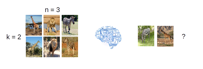 |
| Example of a k-shot problem: the algorithm needs to classify images from 3 classes, with only 2 examples per class available |
The standard deep-learning approach to few shots learning is in fact base on transfer learning where an deep network is trained on a large domain and then it is just fine-tuned on the k-shots domain.
In transfer learning a machine learning model, typically a deep neural network, is pre-trained on a large domain, called the source domain that is related to the domain on which the problem is defined, called the target domain. The pre-trained model last few layers are then re-initialized, while some of the earlier ones are frozen. The model model training then continues on the target domain.
This procedure allows using the pre-trained model as a feature extractor, while using the target domain only to train the high level part of the algorithms.
In the case of image classification one can use state of the art models trained on ImageNet such as VGG, GoogLeNet, Inception or ResNet.
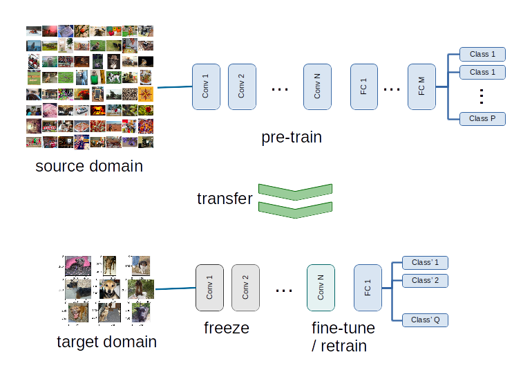 |
| Diagram showing a typical transfer learning setup. A deep neural network is pre-trained on the, large, source dataset, and then it is fine tuned on the target dataset. |
… and zero-shots?
Zero-shots learning is analogous to the case in which you just describe the giraffe to the toddler, but you never show a concrete example.
More formally, in zero shots learning only meta-data are known for each of the n classes.
It is not so complicated to imagine that a transfer learning approach can also be formulated here, provided that meta-data is known in the source domain.
Learning to learn
We are now ready to dive into the learning to learn approach introduced with MatchingNets and PrototypicalNets. The idea behind such approach is to train an algorithm that can fine tune itself on any few-shots domain, without needing to be retrained. In other words, the models being trained are meta models that are trained to learn from any k-shot set.
The models construct a geometric representation of the n classes given the k examples. In such a way, classifying objects reduced to calculating distances between the objects to classify and the classes representation.
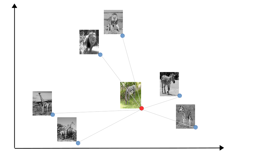
The main difference between MatchingNets and PrototypicalNets is that the former compute distances to each of the examples, while the latter constructs first the center of each of the classes and then compute distances to the class centers. Intuitively, MatchingNets are analogous to k-NN classifiers, while PrototypicalNets are analogous to k-means classifiers.
 |
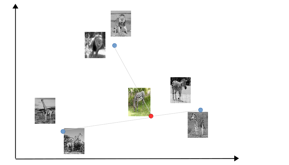 |
| Matching nets approach: the query example is compared to each of the examples in the support set. | Prototype nets approach: the query example is compared to class representations in the support set. |
The big innovation is that the geometric representations are built dynamically for each support set. In standard transfer learning, the models would need to be adapted for each support set trough gradient descent, while in the meta models are trained to already reproduce the results of gradient descent on the support sets.
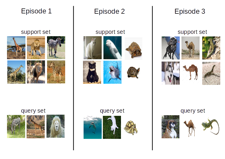
Learning episodes
Let’s now see how can we train a model to learn from small data sets. The procedure involves the generation of several learning epsiodes. In each episode, the network is presented with a k-shots support set, and it is asked to classify a query set with the same class content as the support set.
A set of training and test episodes are constructed, such that the training and test class sets are disjoint.
All the episodes are trained after a baseline classifier has been trained on a large dataset, removing the classes used for few shots learning. The baseline classifier is used as a feature extractor and it is not fine-tuned.
 |
| Learning episodes to train the meta models. |
Embedding functions
The core of the models are the mapping networks that generate the geometric representation of the support and query examples. Both papers construct two independent mappings for the support and query sets.
$g(x_{i}) : S \rightarrow E^{*}$
$f(\hat x) : B \rightarrow E$
Here $x$ are the features extracted by the baseline classifier, while $y$ are the labels.
In the MatchingNets case, the classifier is constructed as
$p(\hat x \vert S) = \frac{1}{|S|} \sum_{x_i \in S} a(\hat x, x_i) y_i$
where $a(\hat x, x_i)$ is an attention field
$a(\hat x, x_i) = e^{ c( g^{T}(x_i), f(\hat x) ) } / \sum_j e^{ c( g^{T}(x_j), f(\hat x) ) } $
Here $c$ is the cosine distance on the embedding space.
In the PrototypicalNets case, a class prototype is constructed by averaging all the class examples.
$c_{a} = \frac{1}{k} \sum_{y_i = a} g(x_i) $
The classifier is then constructed from the softwmax of the Euclidian distance $d$ between the query examples and the class prototypes.
$p_{a}(\hat x \vert S) = e^{ d( c_{a}, f(\hat x) ) } / \sum_b e^{ d( c_b, f(\hat x) ) } $
At this point, it is also easy to see how to extend the prototype approach to the zero-shots case. In the zero shot case, the class description is just available through meta-data information (e.g. length of the neck, color of the hair, etc.).
The class prototypes are defined just in term of meta-data.
$c_{a} = g’(m_a) $
where $m_a$ is the meta-data associated to class a.
The network architectures used by the two approaches are quite different in what concerns the choice of the embedding functions.
The MatchingNets use a bi-directional LSTM to encode the support set and query set examples. In the case of PrototypicalNets a linear mapping is used to go from thee feature sets to the embedding space. In this sense, the PrototypicalNets greately simplifies the MatchingNets, reducing the model to a linear model trained on top of the baseline model.
Summary
The learning to learn approach to k-shots learning is a very interesting development and generalization of the transfer learning concept. It is based on a geometric approach to knowledge representation and generate algorithms that can fine tune their cognitive map without supervision.